Applying Quality Concepts to the Wheel/Rail Interface (Part 2 of 3)
By Stephen S. Woody • January, 2008
Part 1 of this article examined the results of a six-sigma project that Norfolk Southern initiated to improve the efficiency of its grinding program. Part 2 illustrates some the data analysis-related problems that NS experienced and learned from during other six-sigma projects.
One of the most common mistakes made in data analysis is failing to ensure that the data meets the underlying assumptions of a statistical test. When this happens, the analyst may draw a false conclusion from the result. Underlying assumptions to check include whether the:
• data is normal or non-normal.
• variations of each distribution being tested are equal.
• shapes of the distributions being tested are the same.
• number of samples is insufficient, correct, or excessive. (This will be explored in more detail.)
In order for a two-sample “t-test” to be valid, for example, both sample datasets must be normal and the variances must be tested for equality before running the t-test. For another example, the residuals must be normal, independent of each other, and have constant variance for a regression equation to be valid. It is possible to have an invalid regression equation even when the R2 value is high.
Another common mistake made in data analysis is failing to define apractically significant test result as opposed to a statistically significant difference. A practically significant result is one where the difference between sample datasets is large enough to justify action from an economic or technical standpoint.
Take a scenario, for example, in which management wants to know if top-of-rail lubricators should be installed on a route. Assume that the decision will be based on a test of lateral forces on the high rail before and after installing a top-of-rail lubricator at a test site. Also assume that analysis indicates that there is a statistically significant 0.25-kip difference in lateral forces on the high rail before and after lubrication. This means that the distributions of samples taken before and after lubrication are different, and that the high rail forces did change. If, however, the average force reduction must be at least 2 kips in order to justify the cost of the top-of-rail lubricators, then there is no practical difference between the two sample datasets even though there is a statistical difference between them.
A closely related mistake is failing to use an appropriate number of samples for a statistical test. Many wheel/rail practitioners believe that there can never be enough data, and, consequently, take 1,000, 10,000 or even 100,000 samples. Some statistical tests, however, are extremely sensitive to the number of samples used.
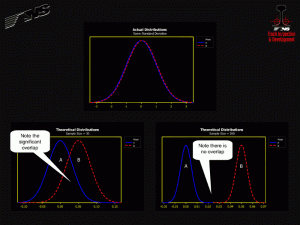
For example, in order to compare the averages of two sample datasets, the statistical test constructs a theoretical distribution of means — called a t-distribution — for each dataset and then checks the amount of overlap of these t-distributions, not the overlap of theactual datasets themselves. If the t-distributions overlap more than a specified amount, the test result will show that there was no statistical difference between the sample datasets. However, the width of each t-distribution and thus the potential for overlap varies with the standard deviation of the actual sample dataset and the number of samples in the dataset.
Figure 1 shows the effect of sample size on statistical testing. The top graph in Figure 1 shows two actual sample datasets. Both distributions are normal and have the same standard deviation. The bottom left graph in Figure 1 shows the t-distribution for each dataset that would result if both sample datasets contained 30 samples. Note that the t-distributions overlap considerably, so the statistical test result should indicate that there is no difference between the two actual distributions. The bottom right graph in Figure 1 shows the t-distributions that would result if both sample datasets contained 200 samples. Note that the t-distributions do not overlap, so the statistical test result should indicate that there is a statistical difference between the two actual distributions. The surprising result is that you can get two different statistical test results for the same data solely due to the number of samples taken.
In order to prevent sample size from influencing the statistical test result, the proper number of required samples should be calculated before testing begins. Many statistical software packages will calculate the correct sample size based on desired inputs. These inputs usually include the amount of difference to be detected (the practically significant difference), the allowable risk for not detecting a difference when one really does exist, and the standard deviation. Be aware that there is a cost to obtaining and analyzing data, and that taking the correct number of samples is the best way to minimize this cost.
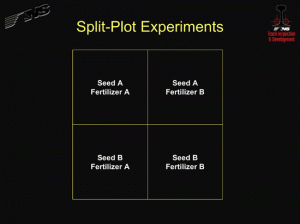
Norfolk Southern has found that a type of statistical analysis called a “split-plot experiment” is often needed in wheel/rail testing. Split-plot experiments originated as a means to compare different agricultural practices, which is a good place to begin an explanation. If I have a garden and I want to see which of two types of seeds and two types of fertilizers produces the best plants, I could subdivide my garden into four equal areas, or plots, and use one type of seed and one type of fertilizer in each area (see Figure 2). I can then measure the plant yield in each plot. However, I cannot determine whether the plant yields in a plot are the result of the seed/fertilizer combination in that particular plot or the result of some characteristic of that particular plot itself.
One or more of the plots may have different soil conditions or receive more sunlight and water than the other plots. The only way that the effects of the seed and the fertilizer can be isolated from the effect of the plot is to further subdivide the garden.
Figure 3 shows each of these plots divided into four sub-plots; the seed and fertilizer has also been varied within each plot. Since I will have a plant yield measurement from each sub-plot, I now have 16 total measurements instead of the four that I had before. Now there are enough measurements to separate the effects of the seeds, the fertilizers, and the plot.
What does this have to do with the wheel/rail interface?
Suppose you want to compare how rail from two different manufacturers wears in track. You could put a piece of rail from manufacturer A in one curve and a piece from manufacturer B in another curve on the same track. In doing so, however, you would not be able to say with certainty whether any difference in wear was due to the rail manufacturer or to some difference between the two track locations. If, however, you put a piece of rail from each manufacture at both track locations (each location is a plot), you could start to attribute how much of the difference in wear was due to the manufacturer and how much was due to the track location. An even better test would be to create subplots (entry spiral, full body, and exit spiral) in each curve with multiple rails from each manufacture randomly placed in each subplot.
For an even more complicated example of a split-plot experiment, consider a truck test that NS recently ran. We equipped each of six cars in a test train with a different type of truck. Then we ran the test train through our test site, which consisted of a lateral force site in two back-to-back curves. We had two measurements for each truck in each curve: the lead measurement and the trail measurement. In effect, each run is a garden, each curve is a plot, each car is a sub-plot and each truck is a sub-sub-plot (see Figure 4).
Since NS also wanted to determine whether the direction of travel affected the truck performance measurements, we wound up with the complicated experiment shown in Figure 5. There are eight gardens for each travel direction. From the experimental setup, there are 192 measurements to analyze, which is enough to separate all of the different factors from each other if the analysis is done properly. The standard statistical analysis for this problem — an ANOVA — would give an incorrect answer because it assumes that the degrees of freedom are the same for all factors. But the degrees of freedom for each variable are not the same in a split-plot experiment. As a result, a modified ANOVA must be used to get the correct answer. Again, it is important to ensure that the data meets the underlying assumptions of the statistical test.
There are a number of ways to make mistakes during data analysis that can cause the analyst to draw an incorrect conclusion. The analyst must gather the correct amount of data, use the correct statistical tests, and verify that assumptions for each test are met in order to draw a correct practical conclusion.
![]()
Stephen S. Woody is Manager, Track Inspection & Development, Norfolk Southern.


